Alessandro Morita Enjoying the thermodynamic limit
Listening to spacetime: simulating black hole binaries
- A personal connection to curved spacetime
- Introducing gravitational waves
- The chirp: inspiral, merger, ringdown
- Why numerical relativity? The SXS catalog
- The simulator: what you see and hear
- Closing reflections
A personal connection to curved spacetime
In 2016, I was finishing my master’s degree at the Perimeter Institute for Theoretical Physics in Waterloo, Canada. For 5 years, I had been trying to become a specialist in Einstein’s theory of General Relativity, which for me was the most exciting area of physics: a framework to describe how space and time bend around matter and energy through mathematics, which had predicted things such as black holes and the expansion of universe.
My excitement is then understandable when, in February, I watched the press conference announcing that humanity had, for the first time, observed real black holes merging. There was a palpable sense of history: a prediction made with pen and paper in 1916 by Einstein had been confirmed.
The actual merger was observed in September 14, 2015, when the LIGO detectors picked up a signal from two black holes merging 1.3 billion light-years away. Gravitational waves had finally been directly detected. The signal, named GW150914, lasted about 0.2 seconds and carried information about two black holes, each roughly 30 solar masses, spiraling into each other and merging.
I felt particularly excited about this discovery because, in the previous year, I had spent four months at the Max Planck Institute for Gravitational Physics, in Germany, working on data analysis of simulations black hole binary mergers – the exact phenomenon that LIGO had measured!
The dataset I used at the time was obtained by the SXS Collaboration (Simulating eXtreme Spacetimes group) which has published a catalog of over 4000 simulated binary black hole mergers, each computed by solving Einstein’s full field equations on supercomputers.
My goal at the time was to study how the energies and angular momentua of the binaries evolved during the inspiral and compare with a quasi-analytical method called “effective one-body”, or EOB. The challenge was to investigate how long during the inspiral/merger process this method would work, and whether results would differ a lot due to numerical noise in the data.
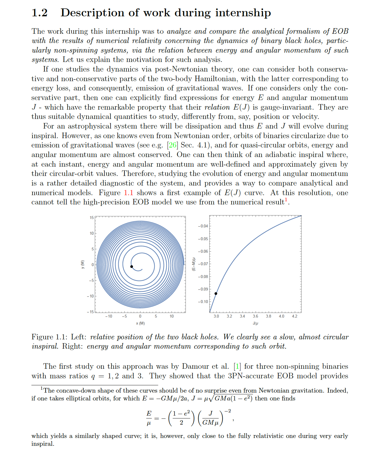 Screenshot of the second page of my final internship report.
My goal in revisiting this dataset was to be able to get a better intuition for how different parameters affect the merger behavior. More specifically, there are a few parameters that can heavily impact the simulation:
- Mass ratio $q$, defined as the ratio between the heaviest and lightest black holes of the binary. By construction, $q>1$.
- Spin directions $\vec \chi_1$, $\vec \chi_2$ of the black holes. These are normalized between 0 and 1, corresponding to black holes rotating with spins $J \le M$. They control precession, or how the orbital plane itself rotates in space.
- Eccentricity $e$: this parameter already exists in Newtonian physics. It represents how far from circular the orbits are.
In this post, I want to walk through the physics: from the basic theory of gravitational waves, through the chirp signal and numerical relativity, to what the simulator actually shows and how it works.
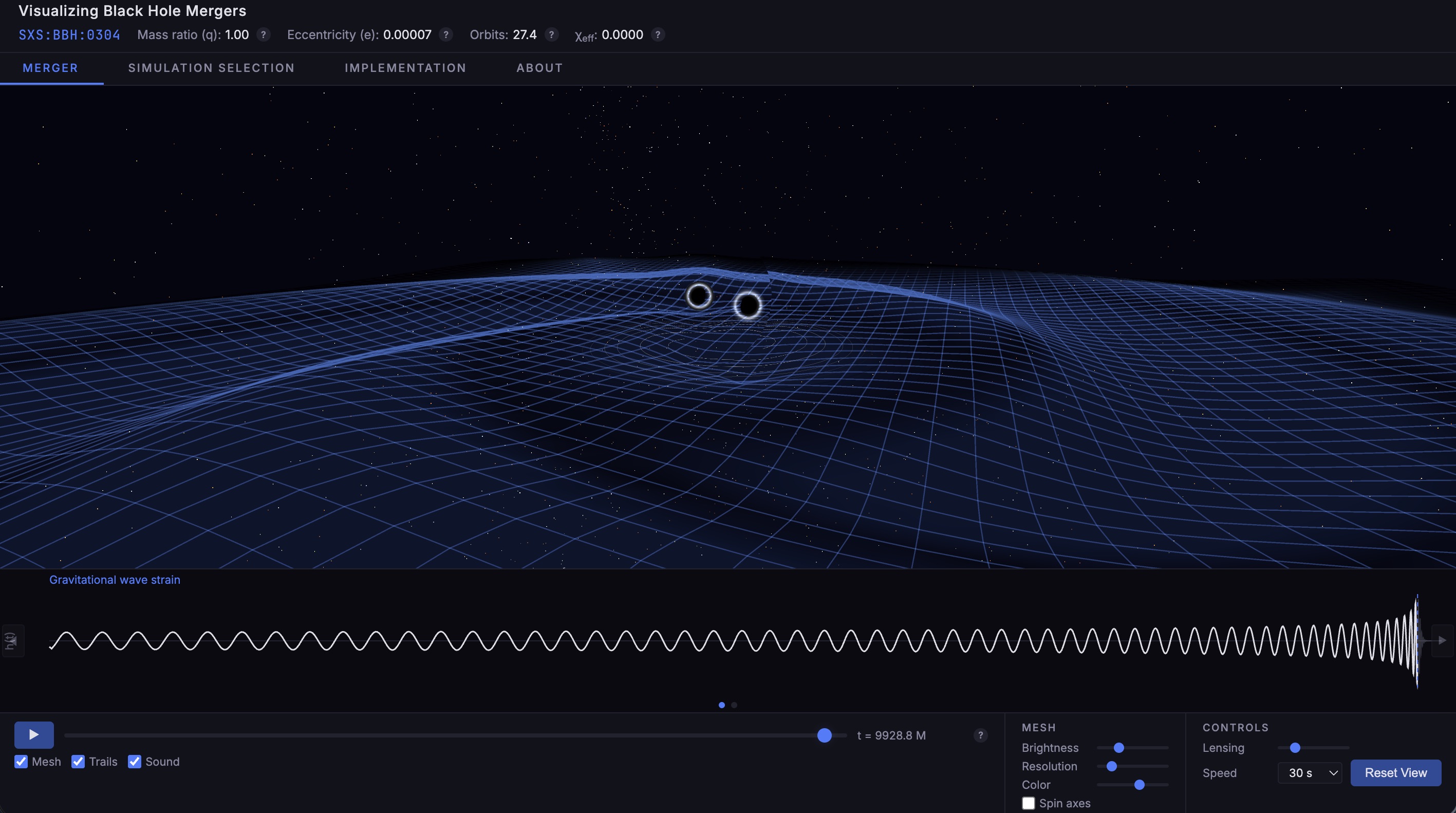
 The simulator showing two black holes mid-inspiral, with gravitational wave ripples propagating outward on the spacetime mesh.
Try the simulator here. You can also check the GitHub repo.
Introducing gravitational waves
Let us start from the beginning: what are gravitational waves, where do they come from, and how do we describe them mathematically?
In special relativity, we are taught that the generalization of the Pythagorean theorem to 4-dimensional spacetime is
\[ds^ 2 = -c^2 dt^2 + dx^2 + dy^2 + dz^2.\]This can be rewritten as the following matrix product:
\[ds^2 = \eta_{ab} dx^a dx^b\]where $\eta_{ab} = \mathrm{diag}(-1, +1, +1, +1)$, and we are summing over indices $a,b$ which run from $x^0=ct$ to $x^3=z$. The tensor $\eta_{ab}$ is called the metric tensor of flat spacetime.
In general relativity, spacetime is posed to be curved and described by a general metric tensor $g_{ab}$, which encodes all information about distances, times, and curvature. When gravity is weak, we can write the metric as a small perturbation around flat (Minkowski) spacetime:
\[g_{ab} = \eta_{ab} + h_{ab}, \quad |h_{ab}| \ll 1.\]The tensor $h_{ab}$ is a perturbation. Plugging this into the Einstein field equations and keeping only terms linear in $h_{ab}$, one obtains a remarkable result: a wave equation
\[\Box \bar{h}_{ab} = -\frac{16\pi G}{c^4}\, T_{ab}\]where $\Box = -\frac{1}{c^2}\frac{\partial^2}{\partial t^2} + \nabla^2$ is the d’Alembertian operator and $T_{ab}$ is the stress-energy tensor.
This is obtained after choosing a convenient gauge (the Lorenz gauge, $\partial^a \bar h_{ab} = 0$, where $\bar h_{ab} = h_{ab} - \frac{1}{2}\eta_{ab}h$ is the trace-reversed perturbation)
This equation is structurally identical to the equations governing electromagnetic radiation. The source term $T_{ab}$ plays the role of the current density in Maxwell’s equations. Gravitational disturbances propagate as waves at the speed of light, $c$, just as electromagnetic waves do.
The quadrupole formula
Solving the wave equation in the far-field limit (far from the source) gives the celebrated quadrupole formula. Just as electromagnetic radiation is dominated by the dipole moment of a charge distribution, gravitational radiation is dominated by the so-called quadrupole moment.
Define the mass quadrupole moment tensor as
\[I_{ij}(t) = \int \rho(t, \mathbf{x})\, x_i x_j \, d^3x\]where $\rho$ is the mass density. Then the gravitational wave strain far from the source is:
\[\boxed{h_{ij}^{TT}(t, \mathbf{x}) = \frac{2G}{c^4 r}\, \ddot{I}_{ij}^{TT}(t_{\text{ret}})}\]Here $r$ is the distance to the source, $t_{\text{ret}} = t - r/c$ is the retarded time (accounting for the finite speed of propagation), and $TT$ denotes the transverse-traceless projection — gravitational waves are transverse (perpendicular to the direction of propagation) and traceless, just like electromagnetic waves in the radiation gauge.
Polarizations of a circular binary
The quadrupole formula, while general, is most illuminating when applied to a specific system. The textbook example is a Newtonian binary system of masses $m_1$ and $m_2$ in a circular orbit — exactly the configuration relevant for binary black holes.
Let the binary orbit in the $(x,y)$ plane. Classical mechanics teaches us that the dynamics of the system is equivalently represented by a sum of two independent components: the center of mass, of mass $m_1+m_2$, in uniform rectilinear motion, and a body with mass $\mu = m_1 m_2 / (m_1 + m_2)$ (called the reduced mass) moving along a circle of radius $R$ around the center of mass. Fixing the center of mass, one finds
\[I_{xx} = \mu R^2 \cos^2(\omega_{\text{orb}} t), \quad I_{yy} = \mu R^2 \sin^2(\omega_{\text{orb}} t), \quad I_{xy} = \mu R^2 \cos(\omega_{\text{orb}} t)\sin(\omega_{\text{orb}} t)\]where $\omega_\text{orb} = \sqrt{G(m_1+m_2)/R^3}$ is the orbital frequency.
Taking two time derivatives (and applying the TT projection for an observer along the $z$-axis), the quadrupole formula yields two independent gravitational wave polarizations:
\[h_+(t) = \frac{4G\mu}{c^4 r}\,(\omega_{\text{orb}} R)^2\,\frac{1+\cos^2\iota}{2}\,\cos(2\omega_{\text{orb}} t_{\text{ret}})\] \[h_\times(t) = \frac{4G\mu}{c^4 r}\,(\omega_{\text{orb}} R)^2\,\cos\iota\,\sin(2\omega_{\text{orb}} t_{\text{ret}})\]where $\iota$ is the inclination angle between the orbital angular momentum and the line of sight. Notice the factor of $2$: the gravitational wave oscillates at twice the orbital frequency.
Using Kepler’s third law $\omega_{\text{orb}}^2 = G(m_1+m_2)/R^3$, the strain amplitude can be written purely in terms of the orbital frequency and the chirp mass:
\[h \sim \frac{4}{r}\left(\frac{G\mathcal{M}}{c^2}\right)^{5/3}\left(\frac{\pi f_{\text{GW}}}{c}\right)^{2/3}\]which shows that higher-frequency waves are also stronger — the signal gets both louder and higher-pitched as the binary spirals in.
How gravitational waves affect matter
Before moving on, let us address one important physical question: how does a passing gravitational wave actually affect matter?
The answer lies in the name “strain” — $h$ measures the fractional change in distance between freely falling test masses. If two masses are separated by a distance $L$, a passing gravitational wave changes their separation by $\Delta L = \frac{1}{2} h\, L$. A gravitational wave passing through a ring of test particles alternately stretches and squeezes them along perpendicular axes:
- The $+$ polarization stretches along $x$ while squeezing along $y$, then reverses.
- The $\times$ polarization does the same thing, but rotated by $45°$.
This is the principle behind LIGO: each detector has two 4 km arms at right angles. A passing gravitational wave makes one arm slightly longer and the other slightly shorter, and the laser interferometer measures the resulting phase shift in the reflected light. For GW150914, the maximum strain was $h \approx 10^{-21}$ — meaning the 4 km arm length changed by about $\Delta L \approx 4 \times 10^{-18}$ m, roughly a thousandth the diameter of a proton. The fact that this can be measured at all is one of the great technical achievements of modern physics.
To achieve this sensitivity, LIGO uses 40 kg mirrors suspended as pendulums (to isolate them from ground vibrations), 200 W lasers with power recycling (to boost the effective power to hundreds of kW circulating in the arms), and a vacuum system that keeps the entire 4 km beam path at $10^{-9}$ torr. The engineering challenges are as impressive as the physics.
The chirp: inspiral, merger, ringdown
Three phases of coalescence
The gravitational wave signal from a binary black hole merger has a distinctive shape that tells the entire story of the event. It is conventionally divided into three phases:
-
Inspiral — The two black holes orbit each other, slowly losing energy to gravitational radiation. As they lose energy, they spiral inward: the orbit shrinks, the orbital velocity increases, and the gravitational wave frequency and amplitude both rise. This is the chirp: a signal that sweeps upward in frequency, like a bird’s call.
-
Merger — When the black holes get close enough (roughly at the innermost stable circular orbit), the slow inspiral gives way to a violent plunge. The two horizons touch and merge into one. This is the peak of the gravitational wave signal — the moment of highest amplitude and frequency.
-
Ringdown — The newly formed, distorted black hole settles down to a stationary Kerr black hole by radiating away its asymmetries as quasi-normal modes. These are damped oscillations: the gravitational wave signal rings like a struck bell, with exponentially decaying amplitude.
The figure-skater analogy works well here: as the skater pulls her arms in, she spins faster. Similarly, as the orbit shrinks, the black holes orbit faster, emitting gravitational waves at ever-higher frequency. The “chirp” name comes directly from this frequency evolution — if you could hear it (and, as we will see, you almost can), it would sound like a rising whistle, ending in a brief, sharp tone.
The transition between inspiral and merger happens roughly at the innermost stable circular orbit (ISCO) — the smallest orbit where a test particle can stably orbit a black hole. For a non-spinning (Schwarzschild) black hole, this is at $r_{\text{ISCO}} = 6GM/c^2$, three times the Schwarzschild radius. Inside this radius, there are no stable circular orbits; the inspiral becomes a plunge.
Energy loss and the chirp mass
Why does the frequency rise? Because the binary is losing energy. Gravitational waves carry energy away from the system, and since the binary’s energy is negative (bound orbit), losing energy means the orbit shrinks. A smaller orbit means a faster orbital frequency, which means stronger gravitational wave emission, which means faster energy loss — a runaway process that ends at merger.
The power radiated as gravitational waves by a circular binary was computed by Peters and Mathews (1963):
\[\frac{dE}{dt} = -\frac{32 G^4}{5 c^5}\,\frac{m_1^2\, m_2^2\, (m_1+m_2)}{R^5}.\]Notice the $R^{-5}$ dependence: as the separation halves, the radiated power increases by a factor of 32. This is the engine behind the chirp.
The formula makes another important prediction: the binary’s evolution is governed by a specific combination of the component masses called the chirp mass:
\[\boxed{\mathcal{M} = \frac{(m_1\, m_2)^{3/5}}{(m_1 + m_2)^{1/5}}}\]The chirp mass gets its name precisely because it determines the rate at which the frequency chirps — sweeps upward. To leading (Newtonian) order, the gravitational wave frequency evolves as
\[f_{\text{GW}}(t) \propto (t_{\text{merger}} - t)^{-3/8}\]which diverges as $t \to t_{\text{merger}}$: the frequency formally goes to infinity at merger. In reality, the post-Newtonian approximation breaks down well before this point, and one needs numerical relativity to follow the evolution through the merger.
From the Peters formula, one can also derive the time remaining until merger for a circular binary with separation $R$:
\[t_{\text{merge}} = \frac{5\,c^5}{256}\,\frac{R^4}{G^3\, m_1\, m_2\,(m_1+m_2)}.\]For the Hulse-Taylor binary pulsar (the first system where gravitational wave energy loss was observed, earning Hulse and Taylor the 1993 Nobel Prize), this formula predicts merger in about 300 million years — a long time, but cosmologically imminent.
The chirp mass is the best-measured parameter from a gravitational wave observation. LIGO can typically determine $\mathcal{M}$ to better than $0.1\%$ accuracy from the inspiral signal alone. This is because the chirp mass enters the phase evolution of the waveform at the lowest (Newtonian) order, and LIGO is exquisitely sensitive to the phase.
Ringdown
After the merger, the remnant black hole is initially highly deformed. It relaxes to a Kerr (spinning) black hole by emitting gravitational waves at its quasi-normal mode frequencies — complex frequencies $\omega = \omega_R + i\, \omega_I$, where the real part gives the oscillation frequency and the imaginary part gives the exponential damping rate:
\[h(t) \sim A\, e^{-t/\tau}\, \cos(\omega_R\, t + \phi_0), \quad t > t_{\text{merger}}\]The quasi-normal mode frequencies depend only on the mass and spin of the final black hole — a beautiful consequence of the black hole no-hair theorem. Measuring them tests whether the remnant is truly a Kerr black hole as predicted by general relativity.
If black holes are the “hydrogen atoms” of general relativity (as people like to say), then quasi-normal modes are their spectral lines. Just as measuring hydrogen’s emission lines confirmed quantum mechanics, measuring a black hole’s quasi-normal modes tests GR in the strong-field regime. LIGO has already seen hints of the ringdown in several events — it is one of the most active areas of current research.
Why numerical relativity? The SXS catalog
When pen and paper run out
The quadrupole formula and its post-Newtonian extensions (systematic corrections in powers of $v/c$) work beautifully during the early inspiral, when the black holes are far apart and moving slowly compared to the speed of light. The post-Newtonian expansion has been pushed to extraordinary precision — 4PN order and beyond — and is essential for LIGO data analysis, where it provides fast template waveforms for matched filtering.
But as the binary approaches merger, the gravitational field becomes intensely strong and highly dynamical. The compactness parameter $GM/(Rc^2)$ approaches unity, orbital velocities approach $c$, and the perturbative expansion in $v/c$ breaks down entirely. No analytic method can reliably follow the evolution through the last few orbits, the plunge, and the ringdown.
To follow the evolution through merger and ringdown, one must solve the full, nonlinear Einstein field equations:
\[R_{ab} - \frac{1}{2}\,g_{ab}\,R = \frac{8\pi G}{c^4}\,T_{ab}\]These are ten coupled, nonlinear partial differential equations for the metric $g_{ab}$. For two black holes in vacuum ($T_{ab} = 0$), this reduces to
\[R_{ab} = 0\]— ten vacuum equations that are deceptively simple to write down but enormously difficult to solve numerically. The difficulty stems from their nonlinearity: gravitational waves themselves carry energy, which in turn generates more gravity. The gravitational field sources itself. There is no background spacetime to work with — the spacetime is the dynamical variable.
An analogy: Newtonian gravity is perfectly fine for launching a rocket to the Moon. But for two black holes colliding at a significant fraction of the speed of light, where spacetime itself is being violently deformed, you need the full nonlinear theory — and a supercomputer.
A brief history
The numerical solution of the binary black hole problem was one of the grand challenges of computational physics. The fundamental approach is the ADM formalism (named after Arnowitt, Deser, and Misner): decompose four-dimensional spacetime into a foliation of three-dimensional spatial slices, labeled by a time coordinate $t$. On each slice, the spatial metric $\gamma_{ij}$ and the extrinsic curvature $K_{ij}$ (measuring how the slice is embedded in 4D spacetime) are evolved forward in time. The Einstein equations split into:
- Constraint equations: conditions that must be satisfied on each spatial slice (analogous to $\nabla \cdot \mathbf{E} = \rho$ in electromagnetism)
- Evolution equations: how $\gamma_{ij}$ and $K_{ij}$ change from one slice to the next
The decomposition also introduces two gauge functions — the lapse $\alpha$ (how fast coordinate time advances relative to proper time) and the shift vector $\beta^i$ (how spatial coordinates move from slice to slice). Choosing these gauge functions wisely turned out to be the key to long-term numerical stability. Poor gauge choices lead to coordinate singularities, grid stretching, or exponentially growing errors that crash the simulation within a few orbits.
This reformulation turns the Einstein equations into an initial-value problem that can, in principle, be solved on a computer — typically using finite-difference or spectral methods on adaptive mesh refinement (AMR) grids, with the black hole singularities either excised (cut out of the computational domain) or represented as “punctures” that can move through the grid.
Despite decades of effort, stable long-term evolution of binary black holes eluded researchers until 2005, when Frans Pretorius achieved the first successful simulation of a binary black hole inspiral, merger, and ringdown. Shortly after, two other groups independently developed the “moving puncture” method, opening the floodgates of numerical relativity. Within a few years, groups around the world were routinely simulating binary black hole mergers, and the race to build comprehensive catalogs began.
The timing was extraordinarily fortunate: the first numerical relativity waveforms became available just a few years before LIGO’s first detection in 2015. Without them, the collaboration would not have had accurate template waveforms for the merger and ringdown phases — and extracting the source parameters from GW150914 would have been far less precise.
The SXS Catalog
The SXS Collaboration (Simulating eXtreme Spacetimes) has since built the largest public catalog of numerical relativity simulations: over 4,150 binary black hole mergers, spanning a wide range of physical parameters:
- Mass ratio $q = m_1/m_2$: from equal-mass ($q = 1$) to extreme ratios ($q > 10$)
- Spin vectors $\vec{\chi}_1, \vec{\chi}_2$: the dimensionless spin of each black hole (magnitude between 0 and 1, in any direction)
- Eccentricity: from quasi-circular to eccentric orbits
- Number of orbits: from short (~10 orbits) to long (~150 orbits) simulations
Each simulation represents thousands of CPU-hours of computation, producing detailed output: the gravitational waveform $h(t)$ (decomposed into spherical harmonic modes), black hole trajectories, black hole trajectories (positions and velocities as functions of time), and the evolution of physical quantities like radiated energy, angular momentum, and orbital separation. My simulator uses a curated selection of 50 of these simulations, precomputed and stored as JSON files for fast browser-side loading.
What does the parameter space look like? Each simulation is characterized by at least 7 intrinsic parameters: the mass ratio $q$, six spin components ($\vec{\chi}_1$ and $\vec{\chi}_2$), and the eccentricity. A commonly used derived quantity is the effective spin:
\[\chi_{\text{eff}} = \frac{m_1\,\chi_{1z} + m_2\,\chi_{2z}}{m_1 + m_2}\]which measures the mass-weighted projection of the spins along the orbital angular momentum. Systems with large positive $\chi_{\text{eff}}$ (spins aligned with the orbit) inspiral more slowly and radiate less energy; anti-aligned spins ($\chi_{\text{eff}} < 0$) lead to faster mergers.
As an example: the default simulation in the app, SXS:BBH:0304, is an equal-mass binary with anti-aligned spins ($\chi_1 = +0.5$, $\chi_2 = -0.5$, giving $\chi_{\text{eff}} \approx 0$), completing about 27 orbits before merging. The remnant black hole has mass $\approx 0.952\,M$ (about 4.8% of the total mass was radiated as gravitational waves) and dimensionless spin $\approx 0.686$.
The simulator: what you see and hear
The Black Hole Binary Simulator is a Three.js application that visualizes the numerical relativity data in real time. It is built with vanilla JavaScript and Vite, and runs entirely in the browser — no server-side computation needed. The pre-processed simulation data (waveforms, trajectories, evolution quantities) is stored as static JSON files and cached in the browser’s session storage for fast switching between simulations.
Let me walk through each visual and auditory element and the physics behind it.
The main visualization consists of:
- A deformable spacetime mesh showing the curvature of space
- Two black hole spheres with glow halos and spin arrows
- Orbital trails tracing the past 300 positions of each black hole
- Gravitational lensing distorting the scene near each black hole
- A chirp audio track synthesized from the waveform data
- Real-time waveform and evolution plots
Spacetime mesh deformation
The most prominent visual element is the deformable spacetime mesh: a grid that warps in response to the gravitational field. The deformation has two components, representing two different physical regimes.
Near zone: gravity wells. Close to each black hole, the mesh dips down to represent the deep gravitational potential. The depth is proportional to the black hole mass, with a Gaussian envelope that smoothly confines the well to a region comparable to the orbital separation:
\[z_{\text{well}} = -\sum_{A=1,2} \frac{\alpha\, m_A}{|\mathbf{x} - \mathbf{x}_A| + \epsilon}\,\exp\!\left(-\frac{|\mathbf{x} - \mathbf{x}_A|^2}{4\,d^2}\right)\]where $\alpha$ is a visual scale factor, $\epsilon$ is a softening parameter (to prevent divergence at the black hole position), and $d$ is the binary separation. This is essentially a softened Newtonian potential with a Gaussian cutoff — not the true Schwarzschild geometry, but a faithful visual representation.
Wave zone: quadrupole radiation. Away from the binary, the mesh shows outgoing gravitational waves with the characteristic quadrupole (spin-2) radiation pattern:
\[\boxed{z_{\text{wave}} \propto \frac{h(t)}{r_{\text{COM}}}\,\cos\!\big(2\phi - \phi_{\text{ret}}\big)}\]where $r_{\text{COM}}$ and $\phi$ are polar coordinates from the center of mass, $h(t)$ is the waveform amplitude from the numerical relativity data, and $\phi_{\text{ret}} = \phi - 2\pi f_{\text{GW}}\,(r_{\text{COM}}/c_{\text{prop}})$ is the retarded phase accounting for the finite propagation speed. The $\cos(2\phi)$ factor encodes the quadrupole pattern: the wave has two lobes (maxima and minima at $90°$ intervals), consistent with the spin-2 nature of the graviton.
Think of it as a rubber sheet with two heavy dents (the black holes), connected by a bridge of deformed spacetime, with spiral ripples propagating outward from the center — getting weaker as they spread, but carrying energy to infinity.
The mesh uses an $81 \times 81$ Cartesian grid (rather than polar coordinates, to avoid aliasing and pole artifacts). The vertex colors are mapped from displacement magnitude, giving an intuitive heat-map of where the spacetime deformation is strongest: deep blue in the gravity wells, bright cyan at the wave crests.
Gravitational lensing
Black holes bend light. This is one of the most visually striking predictions of general relativity, first confirmed during the solar eclipse of 1919 when Arthur Eddington measured the deflection of starlight passing near the Sun.
For a black hole, the effect is far more dramatic. The classical deflection angle for light passing a mass $M$ at impact parameter $b$ is
\[\alpha = \frac{4GM}{c^2 b}\]which diverges as $b \to 0$: light passing arbitrarily close to the event horizon can orbit the black hole multiple times before escaping. This creates a bright ring of light — the Einstein ring — and the distinctive visual distortion seen in images of black holes (made famous by the movie Interstellar and, more recently, by the Event Horizon Telescope).
The simulator implements gravitational lensing as a post-processing shader. Each pixel is displaced toward the black hole by an amount
\[\delta = \frac{s\, r_{\text{EH}}^2}{\rho^2 + r_{\text{EH}}/2}\]where $\rho$ is the distance from the pixel to the black hole center (in screen coordinates), $r_{\text{EH}}$ is the event horizon radius, and $s$ is a strength parameter. To prevent artifacts and unrealistic distortions near the center, a soft saturation is applied:
\[\delta_{\text{eff}} = \frac{\delta\,\rho}{\delta + \rho + \varepsilon}\]This ensures that no matter how strong the lensing, the effective displacement never exceeds the actual distance to the black hole — light is bent, but it is never “teleported” past the center. Mathematically, one can verify that $\delta_{\text{eff}}$ is a monotonically increasing function of both the physical deflection $\delta$ and the distance $\rho$, with $\delta_{\text{eff}} < \min(\delta, \rho)$ always. The result is a smooth distortion that grows stronger near the black hole without producing caustic artifacts.
The interplay of the bloom post-processing (giving the black holes their characteristic glow) with the lensing shader creates a visual that, while not physically exact, captures the essential qualitative features: light bending around the black holes, a bright ring near the event horizon, and the warping of the background grid.
Chirp sonification
Perhaps the most visceral feature of the simulator is the sound: you can listen to the gravitational wave chirp.
Real gravitational waves oscillate at frequencies between roughly 10 Hz and a few thousand Hz — tantalizingly close to the range of human hearing (20 Hz to 20 kHz). For stellar-mass binary black holes like those detected by LIGO, the signal sweeps through the audible range during the last fraction of a second before merger. This is no coincidence: the gravitational wave frequency is set by the orbital frequency, which for a binary with total mass $M$ at the innermost stable circular orbit is
\[f_{\text{ISCO}} \approx \frac{c^3}{6^{3/2}\pi G M} \approx 4400\,\text{Hz}\times\left(\frac{M_\odot}{M}\right)\]For a $60\,M_\odot$ system like GW150914, this gives $f_{\text{ISCO}} \sim 75$ Hz — squarely in the audible range. LIGO scientists famously converted the signal to sound; it is a brief, rising “whoop” that has become an iconic representation of the discovery.
In the simulator, the gravitational wave frequency varies across a wide range depending on the simulation. To make every simulation audible, the frequency is linearly mapped to a fixed audible band:
\[\boxed{f_{\text{audio}} = 40 + 760 \times \frac{f_{\text{GW}} - f_{\min}}{f_{\max} - f_{\min}}}\]where $f_{\min}$ and $f_{\max}$ are the minimum and maximum gravitational wave frequencies in the simulation, and the output spans from 40 Hz (a deep bass hum) to 800 Hz (roughly the pitch of a soprano’s high note). This gives 6 octaves of audible range, enough to hear the dramatic frequency sweep.
The chirp is synthesized sample-by-sample at 44.1 kHz (CD quality). The crucial implementation detail is phase integration: rather than simply evaluating $\sin(2\pi f_{\text{audio}}(t) \cdot t)$ at each sample (which would produce artifacts), the phase is accumulated incrementally:
\[\varphi_n = \varphi_{n-1} + 2\pi\, f_{\text{audio}}(t_n)\, \Delta t, \quad \text{chirp}(t_n) = A(t_n)\,\sin(\varphi_n)\]where $A(t_n)$ is the waveform amplitude from the numerical relativity data. This ensures a smooth, continuous frequency sweep without phase discontinuities — the same technique used in FM synthesis. A 30 ms linear fade-in and fade-out prevents audible clicks at the start and end of playback.
Why phase integration matters: if you naively compute $\sin(2\pi f(t) \cdot t)$, the product $f(t) \cdot t$ can have discontinuities in its derivative when $f(t)$ changes rapidly (as it does near merger), producing harsh artifacts. Accumulating the phase sample-by-sample is the correct approach — it is the discrete analogue of the integral $\varphi(t) = \int_0^t 2\pi f(t’)\,dt’$.
The actual gravitational waves from stellar-mass binaries are naturally in the audible range, which is a remarkable coincidence. But each simulation in the catalog has different frequency characteristics, so we rescale to ensure every chirp sounds clear. Close your eyes, hit play, and you are listening to two black holes merging — mapped to sound, but faithful in rhythm and shape to the true waveform.
Waveform and evolution plots
The simulator displays two real-time plots alongside the 3D visualization:
-
Strain waveform $h(t)$. This is the gravitational wave signal itself — specifically, the dominant $(\ell, m) = (2,2)$ spherical harmonic mode of the strain. This is essentially what LIGO measures: the fractional change in length of the interferometer arms as a function of time. The plot shows the characteristic inspiral chirp (slowly rising amplitude and frequency), the sharp peak at merger, and the exponential ringdown.
The waveform is extracted from the SXS simulation data, which provides $h(t)$ decomposed into spin-weighted spherical harmonics
\[{}_{-2} Y_{\ell m}\]The $(2,2)$ mode is the dominant one for non-precessing binaries, containing typically $>90\%$ of the radiated energy. For binaries with significant spin-orbit misalignment (precessing systems), higher-order modes like $(3,3)$ and $(4,4)$ become important — but the $(2,2)$ mode always captures the essential character of the signal.
-
Radiated energy. The second plot shows the cumulative fraction of the binary’s total mass-energy that has been radiated as gravitational waves. It is related to the waveform by
\[E_{\text{rad}}(t) = \frac{1}{16\pi}\int_{-\infty}^{t} |\dot{h}(t')|^2\, dt'\]For a typical equal-mass, non-spinning binary, this reaches about 5% of the total mass — a staggering amount. By comparison, nuclear fusion in stars converts less than 1% of rest mass to energy; black hole mergers are among the most efficient energy-release mechanisms in nature.
To put this in perspective: the GW150914 merger radiated about 3 solar masses of energy as gravitational waves, in about 0.2 seconds. At its peak, the power output was approximately $3.6 \times 10^{49}$ watts — greater than the combined luminosity of all the stars in the observable universe. For a brief moment, two merging black holes outshone everything else.
The radiated energy plot also shows the orbital separation between the black holes, which steadily decreases during the inspiral and drops to zero at merger — a direct visual trace of the binary’s evolution from wide orbit to coalescence.
Exploring the catalog
One of the things I most enjoyed building was the catalog browser. The simulator includes a selection interface that lets you pick from 50 pre-loaded SXS simulations. Each simulation is characterized by its mass ratio, effective spin, eccentricity, and number of orbits. You can sort and filter to find simulations with specific physical properties — for instance, highly spinning black holes, extreme mass ratios, or eccentric orbits.
Some particularly interesting cases to try:
- Equal mass, high spin (e.g., SXS:BBH:0177, $q \approx 1$, $\chi_{\text{eff}} \approx 0.99$): the black holes orbit many times before merging, producing a long, slowly rising chirp. The high aligned spin delays the merger.
- Unequal mass (e.g., $q \approx 3{-}5$): the waveform develops asymmetries — the gravitational wave from the heavier black hole’s motion dominates, and the recoil (gravitational wave “kick”) of the remnant becomes significant.
- Near-zero spin (e.g., SXS:BBH:0304 with $\chi_{\text{eff}} \approx 0$): a “clean” merger where the physics is dominated by the mass ratio alone, making it easier to isolate the effect of mass on the waveform.
Each simulation tells a slightly different story about two black holes meeting their fate — the same underlying physics, but with different characters.
Technical notes
A few implementation details for the technically curious:
- No backend required. The entire application runs client-side. The pre-processed SXS data (waveforms, trajectories, evolution quantities) is stored as static JSON files served by Vite. Session storage caching means that switching between simulations after the first load is nearly instant.
- Rendering pipeline. The Three.js scene renders in two passes: a main pass (black holes, mesh, orbital trails, spin arrows) followed by post-processing (UnrealBloomPass for the glow effect, then the custom lensing shader). An overlay scene renders the halo sprites after lensing, so they remain undistorted — a subtle but important visual choice.
- Waveform interpolation. The SXS data has non-uniform time steps (finer near merger). For playback and audio synthesis, the data is linearly interpolated onto a uniform time grid matching the desired playback duration and sample rate.
Closing reflections
When I first learned general relativity, the subject felt almost unreasonably abstract. Tensor calculus, Christoffel symbols, the Bianchi identity — beautiful mathematics, but far removed from anything one could touch, see, or hear. The detection of gravitational waves changed that. Suddenly, the curvature of spacetime was not just an elegant theoretical framework — it was a measurable, physical phenomenon, recorded as data, converted to sound, and shared with the world.
Building this simulator was my way of making that connection more tangible. It started as a weekend experiment — “can I render a spacetime mesh in Three.js?” — and grew into a project that touches almost every aspect of the physics: waveform extraction, orbital mechanics, wave propagation, lensing, and sonification. The SXS catalog represents decades of computational work — thousands of CPU-hours per simulation, sophisticated numerical methods, and deep theoretical insight. By wrapping that data in an interactive 3D visualization with real-time sonification, I wanted to make it possible for anyone with a web browser to explore what happens when two black holes collide.
There were many delightful moments along the way: the first time the mesh rippled convincingly, the first time I heard the chirp sweep up in pitch, the moment I realized that anti-aligned spins produce a visibly different waveform than aligned spins. Physics comes alive when you can poke at it interactively.
General relativity is often perceived as inaccessible — a subject reserved for specialists with years of mathematical training. And in some sense, this is true: the full theory is technically demanding in ways that few other areas of physics are. But the phenomena it predicts — ripples in spacetime, the merger of black holes, the ringing of a newborn horizon — are viscerally compelling. You do not need to understand tensor calculus to feel the chirp rising in pitch, or to watch two gravity wells spiral together and merge.
There is something deeply satisfying about seeing the mesh ripple, hearing the pitch rise, watching the two black holes spiral inward and merge — and knowing that the waveform driving all of it came from solving Einstein’s equations on a supercomputer.
We live in a remarkable era for gravitational wave astronomy. LIGO and Virgo have now detected nearly 100 binary black hole mergers, and future detectors — LISA in space, the Einstein Telescope underground — will open entirely new frequency bands, revealing supermassive black hole mergers, extreme mass-ratio inspirals, and perhaps phenomena we have not yet imagined. Each detection adds to our understanding of the population of black holes in the universe: their masses, spins, formation channels, and the environments in which they form.
Numerical relativity, web technologies, and open data — these are the ingredients. The SXS catalog is freely available; Three.js and WebGL run on any modern browser; the physics is well understood. The barrier to entry for exploring some of the most extreme phenomena in the universe has never been lower.
If any of this has piqued your curiosity, here are some resources:
- Try the simulator — pick a simulation from the catalog, press play, and explore
- Source code — the full Three.js application
- SXS Gravitational Waveform Database — the full catalog of 4,150+ simulations
- Baumgarte & Shapiro, Numerical Relativity — the standard reference for the field
- Abbott et al., Observation of Gravitational Waves from a Binary Black Hole Merger (PRL 116, 061102, 2016) — the discovery paper
- Peters & Mathews, Gravitational Radiation from Point Masses in a Keplerian Orbit (PR 136, B1224, 1963) — the energy loss formula
- Pretorius, Evolution of Binary Black-Hole Spacetimes (PRL 95, 121101, 2005) — the breakthrough numerical relativity paper
Written on th, by Alessandro Morita