Revisiting quantum mechanics

• Introduction
• The issues
  • Finding a “healthy” domain

(no AI was used to write this text)

Introduction

Quantum mechanics has worked tremendously well for over 100 years. I claim that this has been enabled by a reliable, concise set of notations; in fact, it is my belief that such a notation system allows the scientist to minimize bandwidth dedicated to abstractions, operationalizing via symbolic manipulation. This is in line with Feynman, who says

“(…) do not laugh at notations; invent them, they are powerful. In fact, mathematics is, to a large extent, invention of better notations.” — The Feynman Lectures on Physics, Vol. I

and A. N. Whitehead in his 1911 textbook:

“By relieving the brain of all unnecessary work, a good notation sets it free to concentrate on more advanced problems, and in effect increases the mental power of the race.” — An Introduction to Mathematics

In quantum mechanics, this is largely accomplished by Dirac notation, introduced by Paul Dirac in his The Principles of Quantum Mechanics (1930). Thanks to Dirac notation, and entities such as the Dirac delta function, physicists can mostly neglect many of the technical details of functional analysis in infinite-dimensional spaces, and operate as if doing linear algebra in finite-dimensional ones. It is “powerful and effective beyond any reasonable expectation”, as mentioned by Griffiths in his popular 1995 textbook: indeed, it is remarkable that this formalism does as well as it does given the lack of justification for its formal operations.

In opposition to Dirac, John von Neumann established the rigorous fundamentals of quantum mechanics in his book The Mathematical Foundations of Quantum Mechanics (1932). The power of von Neumann’s formalism, based on the spectral theorem, is that it is fully general, and provides powerful methods for direct and indirect measurements in quantum mechanics.

Von Neumann’s formalism only relies on the theory’s underlying Hilbert space structure, i.e. that of an inner product space which is Cauchy-complete in its natural norm. On the other hand, Dirac’s formalism required decades of work to be formalized: starting with Laurent Schwartz Théory de Distributions (1950), which established the Dirac delta function as a distribution over test functions, followed by the work of Israel Gelfand and collaborators in the 1960’s, until it finally obtained a rigorous foundation.

It was shown that Dirac’s formalism, strictly speaking, cannot exist without expanding or equipping the Hilbert space; this was indeed something that Dirac realized himself, as pointed in his book: “the bra and ket vectors that we now use form a more general space than a Hilbert space”. Today this is called the rigged Hilbert space.

Which formalism should one adopt, then? I think most physicists live in a superposition of both. The philosophy is not far from that of a student faced with an iterated integral: she will happily change the order of integration and see what happens; if it blows in her face, she might take the steps back to validate Fubini’s theorem. Similarly, physicists make heavy use of Dirac’s framework due to its undeniable usefulness; von Neumann himself notes

“Dirac has given a representation of quantum mechanics which is scarcely to be surpassed in brevity and elegance, […].” – The Mathematical Foundations of Quantum Mechanics.

However, it is common knowledge that this may be akin to playing with fire; if necessary, the physicist may put it out by carefully threading in von Neumann’s framework.

In this text, I summarize, for my own record, the key points on how Dirac’s formalism necessitates structure beyond the Hilbert space; how Gelfand and others regularized it; how this approach is equivalent to von Neumann’s earlier theory.

The issues

The following discussion can be seen in almost any introductory books to quantum mechanics.

The setting is a Hilbert space constructed as follows. For any region $\Omega \subseteq \mathbf R^3$, define the set of square-integrable functions

\[\mathcal L^2(\Omega):= \left\{f: \Omega \to \mathbb C \,\Big\vert \, \int_\Omega \vert f\vert^2 d\mu < \infty \right\}.\]

We will set two functions in $\mathcal L^2$ to be equivalent if they differ up to a set of zero measure. Let $[f]$ be a function $f$’s equivalence class. Then, we define the usual Hilbert space for a single particle’s position as

\[L^2(\Omega)=\{[f]: f \in \mathcal L^2(\Omega) \}.\]

A few important things:

• There is no a priori requirement of differentiability here; in fact, functions in $\mathcal L^2$ have no need to even be continuous
• Pointwise evaluation, i.e. computing $f(x)$ for a given $x$, is meaningless in $L^2$. Of course, it makes sense in $\mathcal L^2$, but two functions can be in the same equivalence class but differ at exactly one point. Hence, although $f(x)$ makes sense in $\mathcal L^2$, $f$ makes no sense in $L^2(\Omega)$
• One often interchangeably calls both $L^2$ and $\mathcal L^2$ the “square-integrable functions”. Strictly speaking, this is wrong; the elements of $L^2$ are not functions. We will, too, confound these two, counting on the reader’s ability to tell them apart by the context.

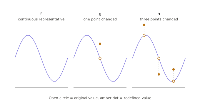Three functions in the same equivalence class, only differing by a zero-measure set

The space $L^2(\Omega)$ is a Hilbert space with inner product \(\langle f, g\rangle_2=\int_\Omega \overline{f(x)}g(x) d\mu(x);\)

note our abuse of notation by writing elements of $L^2$ by representative functions; this is not wrong since these are being fed to an integral and their zero-measure differences do not matter.

Indeed, the “base” $\mathcal L^2$ (with the Lebesgue measure) is not a Hilbert space under this inner product: it allows “too many functions” to have zero norm $\langle f, f\rangle_2$ even though they are not identically zero, namely those that have support on a measure-zero set. This is why we need these (annoying) equivalence classes.

Quantum mechanics poses that the Hilbert space for a single spinless particle bound to a region $\Omega$ is then $L^2(\Omega)$. For more general settings, like many particles, or including spin, the total space would be a (tensor) product of many such $L^2$’s and some finite-dimensional spin spaces; this doesn’t matter much. For our argument, $L^2$ suffices.

Let’s call $L^2(\Omega) = \mathcal H$ from now on.

The axioms of quantum mechanics pose that observables are Hermitian operators in $H$, i.e. operators who equal their adjoints. The adjoint of an operator $A$, denoted by $A^\dag$, is defined via its action on vectors inside the inner product:

\[\langle f, A g\rangle =\langle A^\dag f, g\rangle,\quad \forall f,g, \in \mathcal H.\]

In real, finite-dimensional spaces, this is just the transpose. For complex spaces, it becomes the transpose + complex conjugation, as one can easily see by computing the matrix elements directly on a basis ${e_i}_{i=1}^n$:

\[(A^\dag)_{ij} = \langle e_i, A^\dag e_j\rangle = \langle A e_i, e_j\rangle=\overline{\langle e_j, A e_i\rangle} = \overline{A}_{ji}.\]

Hence, quantum mechanics wants operators satisfying $A^\dag = A$.

Arguably, the two most important operators in quantum mechanics are the position, $X$, and momentum, $P$, whose actions on functions are

\[(Xf)(x):= xf(x);\qquad (Pf)(x) := - i \hbar \frac{\partial f}{\partial x}.\]

In this article, to keep notation clean, I will use capital letters for operators as opposed to hats, as is more common in physics.

We immediately find ourselves with a problem: these are ill-defined expressions.

For starters, we want $X$ and $P$ to act not on functions, but on equivalence classes of functions. As we mentioned before, even if $f(x)$ makes sense, the pointwise evaluation $f$ does not; hence, there is no natural way to define $X[f]$ since the right-hand side doesn’t make sense.

The situation for $P$ is equally problematic: elements of $L^2$ do not have proper notions of derivatives.

Finding a “healthy” domain

What can we do? One way is to start compressing the Hilbert space: if $X[f]$ does not make sense for all $[f] \in \mathcal H$, it may exist a subset $D_1(X) \subset \mathcal H$ such that it does, such as one including continuous functions who are also square-integrable. Then, we can confound $[f]$ and $f$, and $f(x)$ starts making sense again.

… but this does not make the new function $x\mapsto x f(x)$ square-integrable! So now we need to cap again the domain towards a $D_2(X) \subset D_1(X)$ for which $Xf$ is again a function in $\mathcal H$.

This construction can go forever, also considering powers of the operator - we care about computing $X^2 f$ when calculating the variance of position, and so on.

In general, the procedure is as follows. There are at least three operators one really wants to be able to define:

• Position $X$
• Momentum $P$

• The Hamiltonian $H$: this is what describes the dynamics of the system, and what is fed into the Schrodinger equation. In its simplest form it can be written as

  \[H = \frac{P^2}{2m} + \hat V\]

  where $V$ is the potential energy and $P^2/2m$ is the kinetic energy of a particle with mass $m$. $\hat V$ can be very general: it may take position as an argument (think of the harmonic oscillator for which $V = kX^2/2$) or be a new operator by itself; for the case of the electrostatic potential in the hydrogen atom, it is a multiplicative operator\((\hat Vf)(x) := - \frac{1}{4\pi \varepsilon_0} \frac{Qq}{\vert x \vert} f(x)\)

If these three operators are defined, we can do physics and measure things.

First, for any operator $A$, define its domain as:

\[D(A) = \{ f \in H: Af \in H \}.\]

We want a space which is, at the same time, part of $D(X)$, $D(X^2)$, $D(X^3)$ and so on, but also for $D(P^{36})$ or $D(H^3 X^2)$. This means: if I take arbitrary powers of the observables I care about, their domain should be in my final space.

We then construct that space exactly via the following scary expression:

\[\Phi := \bigcap_{\substack{n,m \geq 0\\A, B \in \{X,P,H\}}} D(A^n B^m)\]

In the literature, one often sees a slightly different construction: create a single “Nelson” or control operator” $\Gamma$ and build $\Phi = \bigcap_{n\geq 0} D(\Gamma^n)$ from it alone. More often than not $\Gamma = 1 + X^2 + P^2$ is enough; for cases with singular potentials, more specific constructions are needed.

Written on th, by Alessandro Morita