KakkoKari (仮) Another (data) science blog. By Alessandro Morita
A ROC AUC partial to misclassification cost

This was originally written as a quick intro to partial AUCs, aimed at giving my team at the DataLab some insights into cost-based classification.
Below, we consider the standard binary classification problem.
Assume we pay a cost $c_\mathrm{FN} >0 $ in case we classify a point of the positive class as a negative, and, similarly, pay a cost $c_\mathrm{FP} > 0$ in case of a false positive.
With no loss of generality, we assume these costs are normalized and sum to one:
\[\boxed{c_\mathrm{FN} + c_\mathrm{FP} = 1.}\](if they are not, we can normalize via $c_\mathrm{FN} \to c_\mathrm{FN}/(c_\mathrm{FN} + c_\mathrm{FP})$ and similarly for $c_\mathrm{FP}$).
For a given classification threshold $\lambda \in ]0,1[$, what is the total misclassification cost? Assume we have $n$ total points, out of which $P$ real positives and $N$ real negatives, where
\[P = \pi n, \quad N = (1-\pi) n,\quad \pi \in [0,1] \;\;\mbox{(imbalance ratio).}\]Then the total false positives and false negatives is, written in terms of the coordinates $(\mathrm{FPR}(\lambda), \mathrm{TPR}(\lambda))$ of the ROC curve,
\[\begin{align*} \mathrm{FP}(\lambda) &= N \; \mathrm{FPR}(\lambda)\\ \mathrm{FN}(\lambda) &= P - \mathrm{TP}(\lambda) = P(1 - \mathrm{TPR}(\lambda)); \end{align*}\]multiplying these by the specific costs we get
\[\begin{align*} C(\lambda) &= c_\mathrm{FP} \mathrm{FP}(\lambda) + c_\mathrm{FN} \mathrm{FN}(\lambda)\\ &= c_\mathrm{FP} N\, \mathrm{FPR} (\lambda) + c_\mathrm{FN} P (1 - \mathrm{TPR}(\lambda))\\ &= n c_\mathrm{FP} (1-\pi) \mathrm{FPR} (\lambda) + n c_\mathrm{FN} \pi (1 - \mathrm{TPR}(\lambda)) \\ c(\lambda) \equiv \frac{C(\lambda)}{n} &= (1- c_\mathrm{FN}) (1-\pi) \mathrm{FPR} (\lambda) + c_\mathrm{FN} \pi (1 - \mathrm{TPR}(\lambda)) \quad (*) \end{align*}\]Equation $(*)$ is the general cost at any given $\lambda$.
Now, what is our baseline of comparison? That would be the random model where we set
\[\mathbb P(\hat y = 1) = \pi,\quad \mathbb P(\hat y = 0) = 1 - \pi\]It is easy to see that this model leads to $\mathrm{FPR} = \mathrm{TPR} = \pi$ regardless of the threshold, hence a cost of
\[\begin{align*} c_\mathrm{random} &= (1-c_\mathrm{FN}) (1-\pi) \pi + c_\mathrm{FN} \pi (1-\pi)\\ &= \pi(1-\pi) \end{align*}\]Thus, a good model needs to give a cost lower than random guessing, ie. $c(\lambda) \leq \pi(1-\pi)$, ie.
\[(1- c_\mathrm{FN}) (1-\pi) \mathrm{FPR} (\lambda) + c_\mathrm{FN} \pi (1 - \mathrm{TPR}(\lambda)) \leq \pi(1-\pi)\]or
\[\mathrm{TPR} \geq 1 - \frac{1-\pi}{c_\mathrm{FN}} + \frac{1-c_\mathrm{FN}}{c_\mathrm{FN}} \frac{1-\pi}{\pi} \mathrm{FPR}\]We then arrive at the following criterion:
Cost based partial AUC
- Let $\pi = \widehat{\mathbb P}(Y=1)$ denote the prevalence of the positive class
- Let $\rho \in [0,1]$ denote the cost of a false negative
Then, the region in the $(x,y)$ ROC plane bounded below by
\[\boxed{y = 1 - \frac{1-\pi}{\rho} + \frac{1-\rho}{\rho} \frac{1-\pi}{\pi} x}\]and bounded above by the ROC curve defines the “useful” area from a cost perspective,
Examples and implementation
A “clean” implementation follows after these first examples.
(a) Balanced case
X, y = make_classification(n_classes=2,
                           n_samples=3000,
                           random_state=2,
                           n_features=10,
                           n_informative=10,
                           weights=(0.5,),
                           n_redundant=0,
                           n_repeated=0)

model = LogisticRegression()
model.fit(X, y)

y_probs = model.predict_proba(X)[:,1]

fpr, tpr, thresh = roc_curve(y, y_probs)

pi = y.mean()

for cost_fn in [0.3, 0.5, 0.8]:
    cost_fp = 1 - cost_fn
    rho = cost_fn

    tpr_base = 1 - (1-pi)/rho + (1-rho)/rho * (1-pi)/pi * fpr
    pauc = auc(fpr, np.maximum(tpr-np.maximum(0,tpr_base),0))

    # maximum value
    aux = np.clip(tpr_base,0,1)
    max_pauc = 1 - auc(fpr, aux)


    plt.plot(fpr, tpr_base,
             label=f'FN cost: {cost_fn}\n(pAUC: {round(pauc,2)}\nMaxpAUC: {round(max_pauc,2)})',
             linestyle='--')


plt.plot(fpr, tpr)
plt.xlim(0,1)
plt.ylim(0,1)
plt.legend()
plt.show()

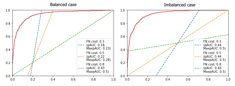
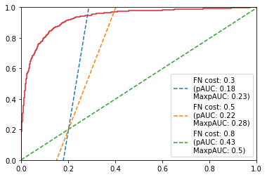
Notice that, in this balanced case, the fact that we are using a cost-based partial AUC doesn’t change much: all AUCs are basically equal.
(b) Imbalanced case
X, y = make_classification(n_classes=2,
                           n_samples=3000,
                           random_state=2,
                           n_features=10,
                           n_informative=10,
                           weights=(0.8,),
                           n_redundant=0,
                           n_repeated=0)

model = LogisticRegression()
model.fit(X, y)

y_probs = model.predict_proba(X)[:,1]

fpr, tpr, thresh = roc_curve(y, y_probs)

pi = y.mean()

for cost_fn in [0.3, 0.5, 0.8]:
    cost_fp = 1 - cost_fn
    rho = cost_fn

    tpr_base = 1 - (1-pi)/rho + (1-rho)/rho * (1-pi)/pi * fpr
    pauc = auc(fpr, np.maximum(tpr-np.maximum(0,tpr_base),0))

    # maximum value
    aux = np.clip(tpr_base,0,1)
    max_pauc = 1 - auc(fpr, aux)


    plt.plot(fpr, tpr_base,
             label=f'FN cost: {cost_fn}\n(pAUC: {round(pauc,2)}\nMaxpAUC: {round(max_pauc,2)})',
             linestyle='--')


plt.plot(fpr, tpr)
plt.xlim(0,1)
plt.ylim(0,1)
plt.legend()
plt.show()

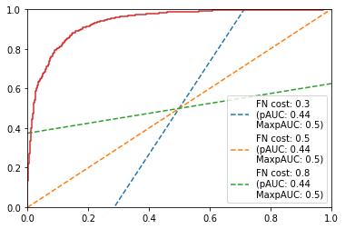
Notice how adding imbalance changes the game significantly.
Functional implementation
Below, as a reference, we leave a function to calculate these metrics following a syntax close to the scikit-learn one.
def cost_based_roc_auc(y_true, y_probs,
                       cost_fn=None,
                       cost_fp=None,
                       return_curves=False):
    from sklearn.metrics import roc_curve, auc

    fpr, tpr, thresh = roc_curve(y_true, y_probs)

    is_fn_none = cost_fn is None
    is_fp_none = cost_fp is None

    assert not all([is_fn_none, is_fp_none]), "At least one out of cost_fn and cost_fp needs to be not None"

    if is_fn_none:
        assert 0 <= cost_fp <= 1
        cost_fn = 1 - cost_fp
    else:
        assert 0 <= cost_fn <= 1

    pi = y_true.mean()

    rho = cost_fn

    tpr_base = 1 - (1-pi)/rho + (1-rho)/rho * (1-pi)/pi * fpr
    pauc = auc(fpr, np.maximum(tpr-np.maximum(0,tpr_base),0))

    # maximum value
    max_pauc = auc(fpr, 1 - np.clip(tpr_base,0,1))

    if not return_curves:
        return pauc, max_pauc
    else:
        return pauc, max_pauc, fpr, tpr, tpr_base
for cost_fn in [0.1, 0.3, 0.5, 0.8, 0.9]:
    pauc, pauc_max = cost_based_roc_auc(y, y_probs, cost_fn=cost_fn)
    print(f"Cost FN {cost_fn}: {round(pauc/pauc_max,2)} %")

# >> Cost FN 0.1: 0.75 %
# >> Cost FN 0.3: 0.76 %
# >> Cost FN 0.5: 0.78 %
# >> Cost FN 0.8: 0.86 %
# >> Cost FN 0.9: 0.9 %